


Google Sheets is a great tool for classroom teachers. It can help you increase your efficiency and organisation. If you’ve never used spreadsheets before they can be a little intimidating, but once you get started I’m sure you’ll realise how powerful Google Sheets really is.
[bctt tweet=”Google Sheets is a great tool for classroom teachers.” username=”lara_kirk”]
Many of the things you’ll want to do in Google Sheets are really straightforward and are done in a similar way to Docs or Slides. However, there are a few things that operate a little differently and can be really frustrating when you first start using this great tool.
Here’s five tips that I wish I’d known when I first started out with Sheets.
PARAGRAPHS IN CELLS
When you have been typing in a cell in Google Sheets and you hit enter, your cursor will move to the next cell. If you want to create paragraphs within a cell you need to hold down command + enter (MAC) or ctrl + enter (PC).
HYPERLINKS
You can create hyperlinks within a sheet in the same way you do in a doc. However, you can’t hyperlink from a multi-paragraph cell. If you really want it to look like multi-paragraphs create your text in seperate cells, link the ones you want, then make the borders between them white.
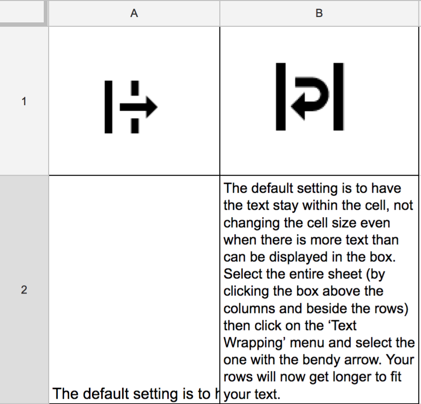
TEXT WRAPPING
The default setting is to have the text stay within the cell, not changing the cell size even when there is more text than can be displayed in the box. Select the entire sheet (by clicking the box above the columns and beside the rows) then click on the ‘Text Wrapping’ menu and select the one with the bendy arrow. Your rows will now get longer to fit your text.
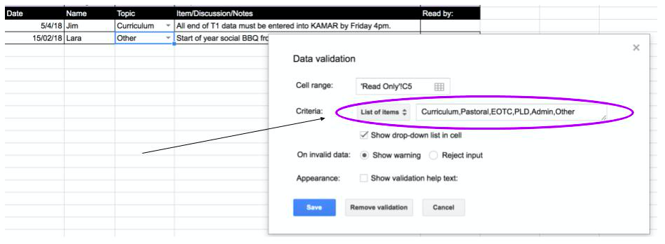
DROP DOWN BOXES
These are great when you want to categorise things or only have a few options. Click in the cell you would like to have the drop down menu, click on the ‘Data’ menu, choose Data validation, change ‘List from a range’ to ‘List of items’ and add your options. You can share this drop down with all cells in the range by dragging the little square at the bottom of the cell (when you’ve selected it) down over the other cells you’d like to apply this to.
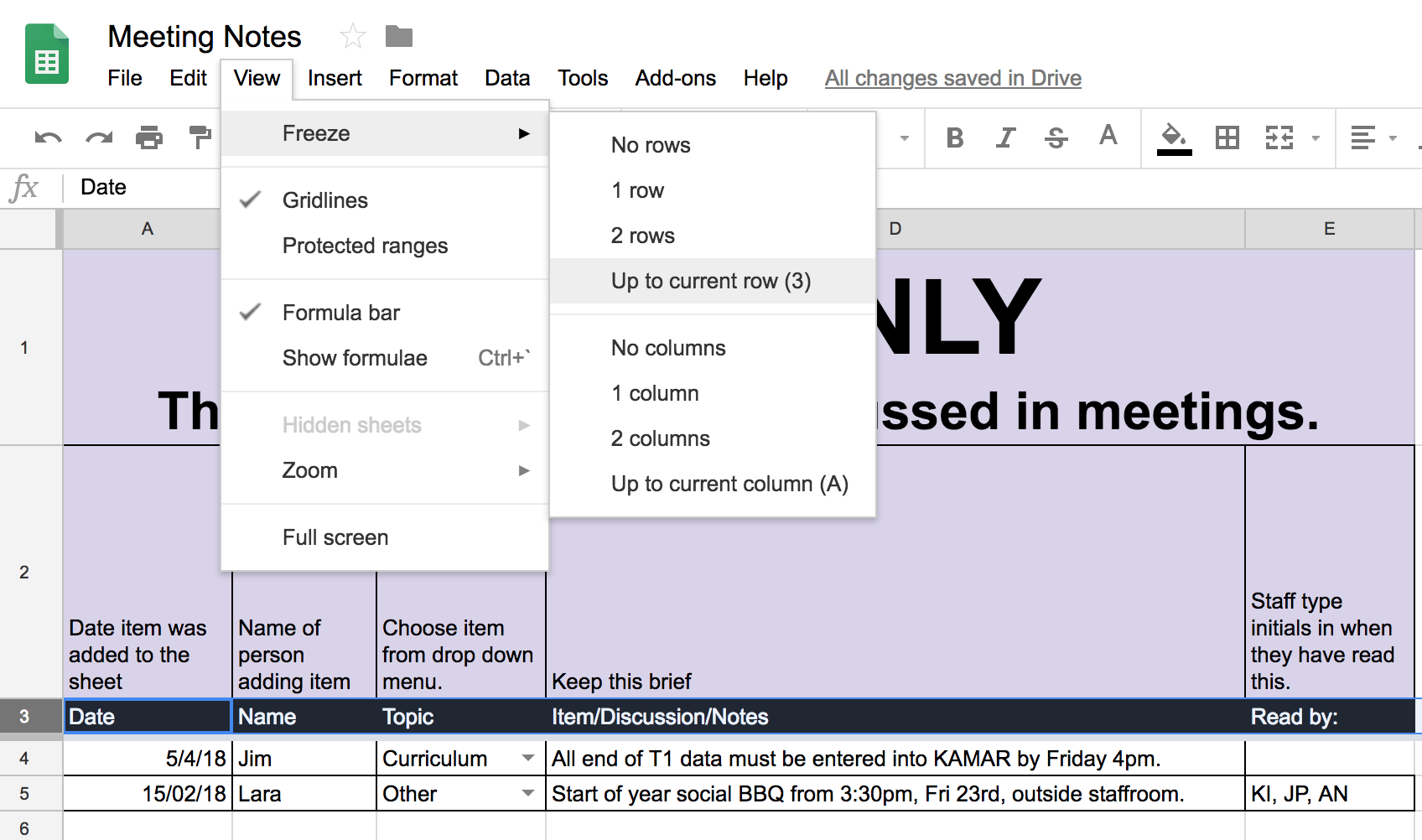
FREEZE ROWS AND COLUMNS
This means that wherever you go on the sheet, or however you sort the sheet, you’ll still be able to see the selected rows and columns. Click in the last column or row that you would like to freeze, go to ‘View’, ‘Freeze’ and select ‘Up to current row’.
[bctt tweet=”5 Google Sheets quick tips to ease your pain!” username=”lara_kirk”]
Check out this blog post to give you some great ideas for how Google Sheets can make you more organised and efficient.
Head over to our web page or download the Using Technology Better app (iOS or Android) to stay up to date with our blog posts and upcoming events.