


By using a simple technique you can make your Google Sheets easier to use by others. Often we create a spreadsheet to carry out a task that we are familiar with so it makes sense to us, but others may struggle with where to enter data and what it represents. This is true for students who we ask to complete a spreadsheet and sometimes they are not sure of what they are entering into a cell. A simple solution to this is to have one column with text, and then enter data in an adjacent cell. What if you could have text and numbers in the same cell and still be able to carry out calculations? We can do this by using custom number formats in Google Sheets.
[bctt tweet=”Learn how to use custom number formats to have text and numbers in the same #Google #Sheets cell and still be able to carry out calculations” username=”adifrancis”]
It may seem like magic, but it is a fabulous function inside Google Sheets that is super easy to set up and can be used in many circumstances. For example, imagine I am wanting to make a spreadsheet where students measure the length of the base of a triangle and the height to calculate the area. I want them to enter the numbers and be aware of what they are measuring. Follow these easy steps to unleash this nifty function and apply it to your own spreadsheets:
1.Click on the cell that you want to use. In this example, I am using cell A3.
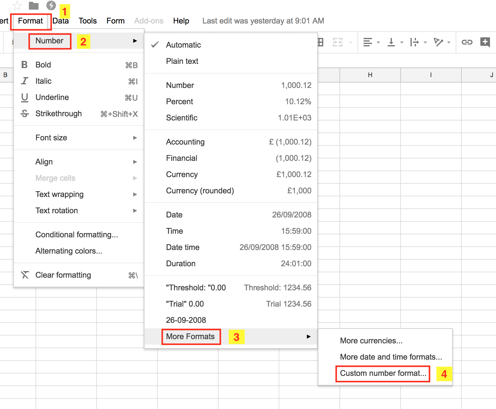
2.Then
- Click on the Format menu.
- Click on Number
- Click on More formats
- Click on Custom number format….
This is where you are able to customise the number format of the cell. Even if you aren’t combining text and numbers, this is a handy menu to be aware of as you are able fully customise the way numbers are entered and displayed. You can even have a number and a date combined in the same cell.
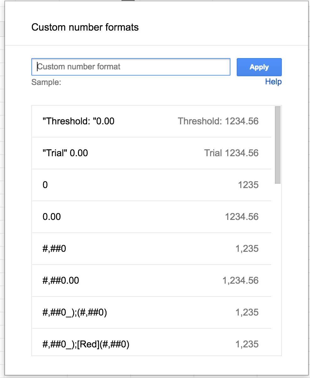
To customise number formats to have text and numbers in a cell:
1.Click on the ‘Custom number format box’
2.Use the following syntax
- text needs to be in quotation marks – In this case, I want the text to read “Length of side A”.
- You also specify how you wish to have the number entered in this case it was with two decimal places 0.00.
A sample of the formatting will be displayed.
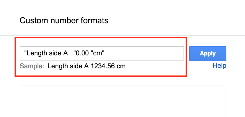
When we do this, the spreadsheet actually recognises the number and ignores the text, allowing us to do calculations.
3.Click Apply to assign this formatting to the cell.
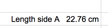
When you look at the spreadsheet it will seem as if nothing has changed. When you enter a number, it looks like any other cell.
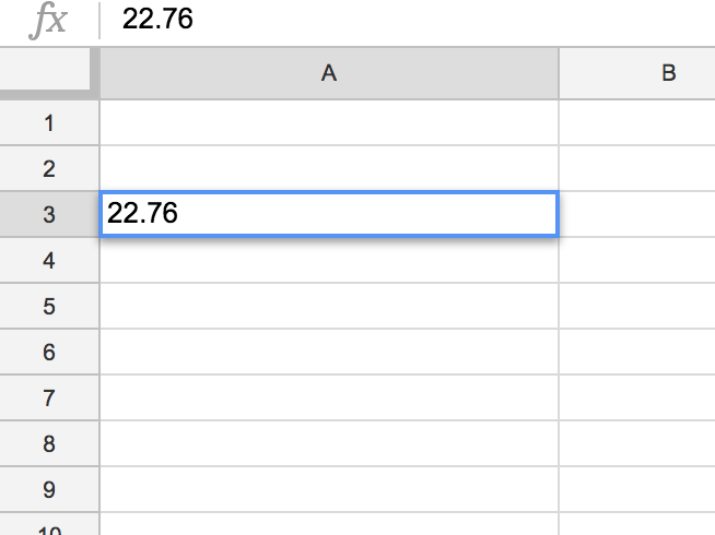
When you hit enter or return on your keyboard, the magic happens and you see this.
You may want to experiment with the spaces and formatting to make it look like you want.
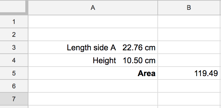
To carry out any calculations, you treat this cell as a normal number cell. I customised another cell with a label of height, then wrote the formula to calculate the area of a triangle.
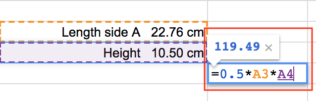
The spreadsheet ignores the text and will carry out any function that you use. It makes it easier for students to understand what they are calculating and also helps others who enter data into a shared sheet.
[bctt tweet=”You will be amazed how this simple #Google #Sheets trick can add clarity to your spreadsheet!” username=”adifrancis”]
This is one of many functions of spreadsheets that go unnoticed. You may be amazed about how useful this can be. To see how to use macros in a Google Sheet click here.